

Internal corrosion quietly thins pipelines from the inside out, draining an estimated US$2.5 trillion from the global economy every year. This article traces the problem from its electrochemical roots to the two field-proven methods — corrosion coupons and electrical-resistance (ER) probes — that turn invisible metal loss into hard, actionable numbers, and closes with a representative field case showing how measurement becomes mitigation.
The scale of the loss is hard to overstate. The NACE International IMPACT study (2016) estimated the global cost of corrosion at US$2.5 trillion per year — about 3.4% of global GDP — and concluded that 15–35% of it (US$375–875 billion) is recoverable with existing practices. In the United States, the direct cost of metallic corrosion runs to US$276 billion annually (3.1% of GDP). Within pipelines specifically, the U.S. Pipeline and Hazardous Materials Safety Administration (PHMSA) found that internal corrosion caused roughly 12% of all pipeline incidents from 1998–2017, and that it accounts for about 60% of all corrosion-caused pipeline incidents. Corrosion is, in short, the single most expensive “invisible” process in the energy supply chain.
But here is the liberating truth: corrosion is measurable. And what is measurable can be managed. The rest of this article follows that chain — from “what corrosion is” and “why it is so costly”, to the two methods operators use to put a number on it.
1. What Is Pipeline Corrosion and Why Does It Cost the Oil & Gas Industry Billions?
1.1 The electrochemical basics
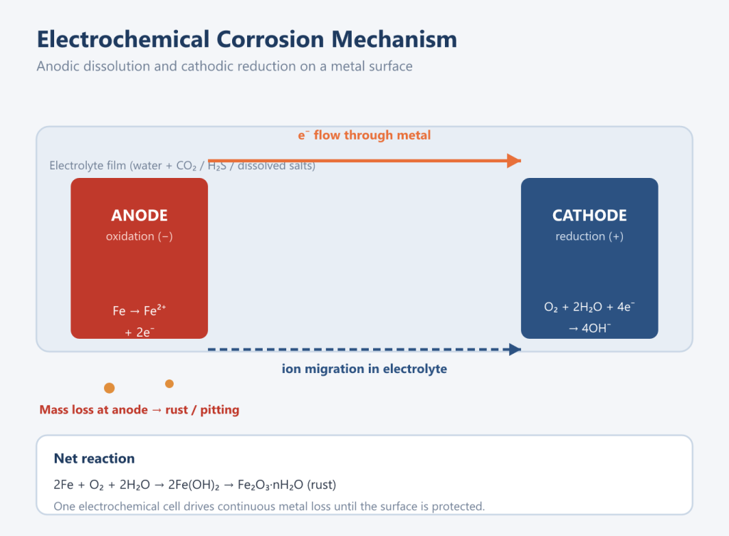
Corrosion is the deterioration of a metal by reaction with its environment. For steel pipelines the dominant mechanism is electrochemical: in the presence of an electrolyte (typically water condensed on the pipe wall), microscopic anodic and cathodic sites form on the metal surface. At the anodes, iron atoms release electrons and enter solution as Fe²⁺ — that is the metal loss. At the cathodes, those electrons are consumed by a reduction reaction (commonly oxygen reduction, or hydrogen evolution in sour, H₂S-rich systems). The two half-reactions are electrically coupled, so as long as the electrolyte, a cathode, and an anode coexist, the steel keeps disappearing.
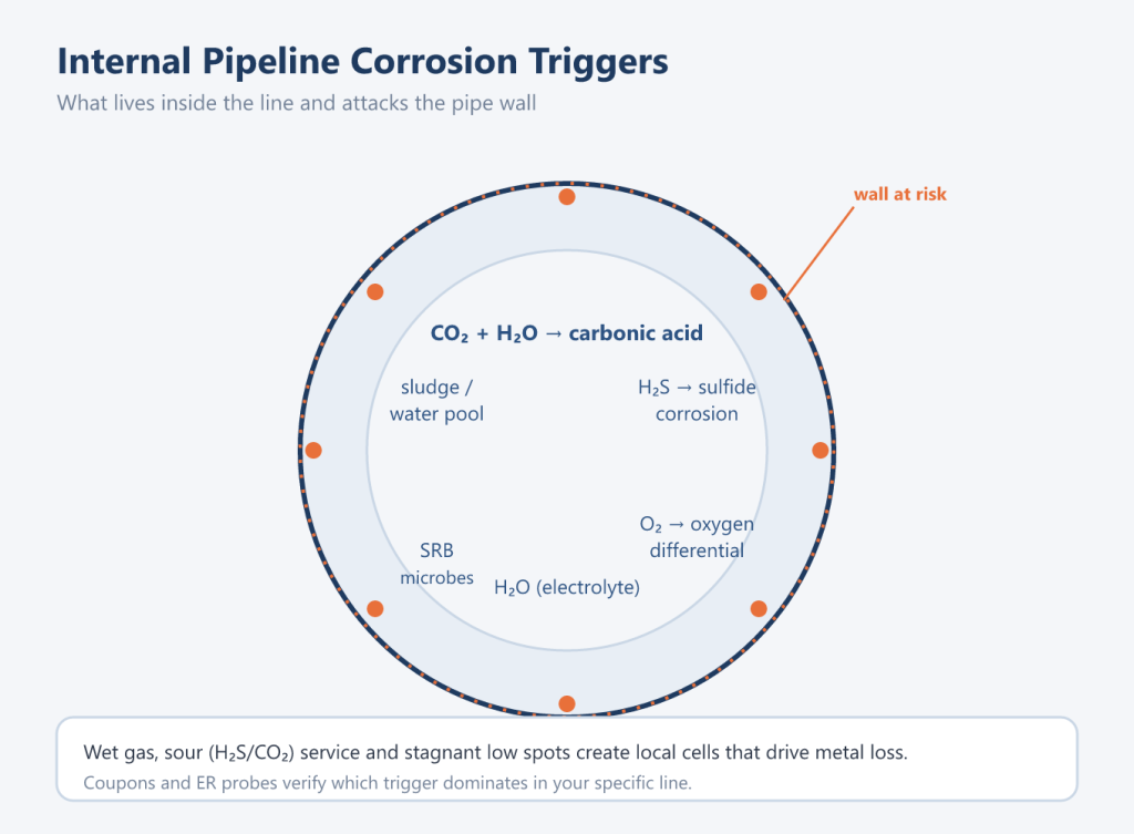
What makes pipelines uniquely vulnerable is that the electrolyte is rarely pure water. Produced fluids are cocktails:
| Species | Common source | Corrosion effect |
| CO₂ (“sweet” corrosion) | Reservoir gas, compression | Forms carbonic acid; can drive uniform rates >10 mm/y in severe, unmitigated cases |
| H₂S (“sour” corrosion) | Sour reservoirs, bacteria | Acid generation **plus** hydrogen embrittlement and sulfide stress cracking risk |
| Free water | Condensation, inadequate dehydration | The electrolyte that makes every other species active |
| O₂ | Air ingress, poor sealing | Extremely aggressive; a few ppm dramatically accelerate rates |
| Cl⁻ | Formation water, seawater | Destroys passive films; drives localized pitting |
| Microbes (MIC) | Sludge, stagnant low spots | Sulfate-reducing bacteria create aggressive local cells under biofilms |
1.2 Why pipelines, specifically
Three features of pipeline service amplify the risk. First, length and inaccessibility — a gathering or transmission line may run hundreds of kilometres, much of it buried or subsea, so a single bad low spot is hard to see. Second, multiphase, changing flow — gas, condensate, and water separate and re-mix, and water settles in low points where it lingers. Third, time dependence — PHMSA classifies internal corrosion as a “time-dependent threat” unlike a third-party dig, it grows worse the longer it is left unmitigated. Early detection is therefore not optional; it is the entire game.
1.3 The bill: what the data shows
The headline figures are sobering and consistent across independent sources:
- Global: US$2.5 trillion/yr (3.4% of GDP) — NACE IMPACT, 2016.
- United States: US$276 billion/yr direct (3.1% of GDP) — FHWA/NACE, 2002; updated by IMPACT.
- Pipelines within that total: PHMSA’s “Pipeline Corrosion Report”attributed about US$7 billion of the US corrosion bill to onshore gas and liquid transmission pipelines, with ~52 significant corrosion incidents per year across 1988–2008, costing 30 fatalities, 100 injuries, and US$551 million in property damage over the period.
- Cause split (liquid pipelines, 2002–2009, API/AOPL): external corrosion 32%, internal corrosion 14% — together nearly half of all liquid-pipeline failures.
- Internal corrosion share: ~12% of all pipeline incidents (1998–2017) and ~60% of corrosion-caused incidents (PHMSA).
1.4 Why the bill is so large
The direct cost of “a little rust” is trivial; the consequential cost is not. A corrosion-driven failure triggers a cascade: lost throughput during shutdown, emergency response and spill containment, environmental remediation, regulatory investigation and potential penalties, unscheduled “integrity digs” to verify wall condition, and reputational damage that outlasts the repair. A single unplanned excavation to inspect a corroding segment can run from tens of thousands to well over a hundred thousand dollars before any steel is even replaced. Multiply across a network, and the trillions add up.
The obvious question follows: *if the loss is measurable and the threat is time-dependent, how do operators actually watch it happen?* The oldest and most trusted answer is also the simplest — put a small piece of the same metal into the line and see what the line does to it.
2. How Corrosion Coupons Work: A Simple Guide to Monitoring Pipeline Health
2.1 What a coupon is — and how it lives in the line
A corrosion coupon is a small, pristine sample of metal — usually the same alloy as the pipe or a deliberate “worst-case” match — machined to a known shape and exposed directly to the process stream. It is mounted in a coupon holder (or “coupon rack”) that threads into an access fitting with an isolation valve, so the coupon can be inserted and retrieved without depressurizing or shutting down the line. In field terms, a retrievable coupon holder lets a technician swap a coupon during normal operation — a capability that matters enormously on continuously running systems.
The principle is elegant: *the coupon is a stand-in for the pipe wall.* Because it sits in the same fluid, at the same temperature and pressure, it corrodes at essentially the same rate as the structure it represents. What the coupon loses, the pipe is losing.
2.2 From exposure to weighing
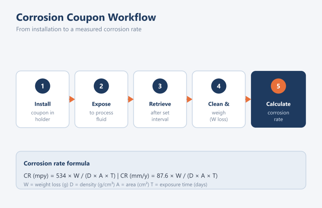
The method is deliberately low-tech and therefore robust:
- Record initial mass W_0 of the clean, dry coupon (typically to 0.1 mg).
- Expose it in the stream for a known interval T (commonly 30–90 days).
- Retrieve and clean it to remove corrosion products without removing base metal (typically by chemical descaling or mild abrasion per ASTM G1 / NACE procedures).
- Weigh again to get final mass W_1.
- Mass loss Δ W = W_0 – W_1 becomes the basis for the corrosion rate.
The only measurements required are mass, area, density, and time — which is precisely why coupons have remained a reference method for decades even as electronics advanced.
2.3 The weight-loss corrosion-rate formula
The corrosion rate is the average penetration of metal per unit time, derived from how much mass was lost over the exposed area. The standard forms are:
In mils per year (mpy):
CR(mpy) = (534 × W) / (D × A × T)
In millimetres per year (mm/y):
CR(mm/y) = (87.6 × W) / (ρ × A × T)
Where:
- W = mass loss (mg)
- D or ρ = density of the coupon metal (g/cm³; e.g. carbon steel ≈ 7.85)
- A = exposed surface area — in² for the mpy form, cm² for the mm/y form
- T = exposure time (hours)
- 534 and 87.6 = unit-conversion constants
More generally, the rate collapses to a single constant form:
CR = (K × W) / (ρ × A × T)
with K chosen for the desired output units:
| Output unit | W | ρ | A | T | K |
| mm/year | mg | g/cm³ | cm² | h | 87.6 |
| μm/year | mg | g/cm³ | cm² | h | 8.76 × 10⁴ |
| mils/year (mpy) | mg | g/cm³ | in² | h | 534 |
| inches/year (ipy) | mg | g/cm³ | in² | h | 0.534 |
2.4 Worked example
A carbon-steel coupon (density ρ = 7.85 g/cm^3) with exposed area A = 10.0 cm^2 is exposed for T = 90 days = 2160 h. Its measured mass loss is Δ W = 0.108 g = 108 mg.
CR(mm/y) = (87.6 × 10⁸) / (7.85 × 10.0 × 2160)
= (9460.8) / (169,)560 ≈ 0.0558 mm/y
Convert to mpy using A = 10.0 cm^2 = 1.55 in^2:
CR(mpy) = (534 × 108) / (7.85 × 1.55 × 2160)
= frac57,67226,291 ≈ 2.19 mpy
The two agree (0.0558 mm/y ÷ 0.0254 ≈ 2.20 mpy), confirming the calculation. A rate near 2 mpy on an inhibited line would typically prompt a review of chemical treatment; on an uninhibited sour service it would be considered mild.
2.5 Reading beyond the average: pitting
Weight loss yields an average rate, but pipelines often fail from localized attack, not uniform thinning. After retrieval, the deepest pit is measured (e.g. with a pit gauge). The pitting rate is then:
PR = fracd(pit)T(years)
where d(pit) is the maximum pit depth and T(years) is the exposure in years. The pitting factor compares localized to uniform severity:
PF = (PR) / (CR)
A pitting factor well above 1 signals that localized corrosion — not the average — governs remaining life, and that mitigation (better inhibitor coverage, water removal, more frequent pigging) must target the worst spots, not just the mean.
Coupons are cheap, direct, and physically truthful: they measure *actual metal removed* by the real fluid. Their weakness is temporality — a coupon yields one number for the whole exposure window. It cannot tell you *when* during those 90 days the corrosion spiked, nor catch a transient upset. For that, operators need a method that watches continuously.
3. ER Corrosion Monitoring Explained: Measuring Metal Loss in Real Time
3.1 The principle
An electrical-resistance (ER) probe places a small sensing element — a wire, strip, or tube of the line metal — directly in the stream, wired to an instrument. The element’s electrical resistance is governed by:
R = ρₑ (L) / (A)
where ρₑ is the element’s resistivity, L its length, and A its cross-sectional area. As corrosion eats into the element, A shrinks and R rises. Measure the resistance continuously and you are, in effect, watching the metal thin in real time.
3.2 The resistance–penetration relationship
For a flat strip element of initial thickness t corroding symmetrically from both faces, the new thickness is t’ = t – 2P, where P is the penetration from one face. Resistance scales inversely with thickness, so:
(R_t) / (R_0) = (t) / (t’) = (t) / (t – 2P)
Solving for penetration:
P = (t) / (2)((R_t) / (R_0) – 1)
The corrosion rate is then penetration divided by the elapsed time:
CR = (P) / (Δ t(exp))
In practice the probe’s instrument applies a built-in geometry constant and reports the rate directly in mpy or mm/y; the equations above are the physical basis. The crucial point is that ER turns a *change in resistance* into a *rate of metal loss* without ever removing the sensor.
3.3 What “real time” buys you
Because the probe reports continuously, it captures trends and transients that a coupon cannot:
- An inhibitor pump trip shows up as an immediate resistance upswing, triggering an alarm within hours rather than at the next coupon pull.
- A process change (new well tied in, slug of water, oxygen ingress) is visible as a slope change, letting operators respond before wall loss accumulates.
- Data can be logged to a historian or wireless gateway, feeding dashboards and predictive alarms.
3.3 What “real time” buys you
Because the probe reports continuously, it captures trends and transients that a coupon cannot:
- An inhibitor pump trip shows up as an immediate resistance upswing, triggering an alarm within hours rather than at the next coupon pull.
- A process change (new well tied in, slug of water, oxygen ingress) is visible as a slope change, letting operators respond before wall loss accumulates.
- Data can be logged to a historian or wireless gateway, feeding dashboards and predictive alarms.
3.4 Coupons vs ER: complementary, not competing
| Dimension | Corrosion coupon | ER probe |
| Output | Average rate over exposure | Continuous rate and trend |
| Detects pitting? | Yes (by pit measurement) | Poorly (measures total area loss) |
| Lag to first reading | One full exposure cycle | Immediate |
| Cost | Very low | Moderate (probe + instrument) |
| Best role | Periodic “ground truth” + pitting check | Early-warning and process monitoring |
Used together, coupons supply the authoritative average and the pitting factor, while ER probes supply the live trend and upset detection. They answer different questions and, combined, leave few blind spots.
Corrosion silently drains an estimated US$2.5 trillion from the global economy every year—roughly 3.4% of GDP—yet much of that loss is preventable. As this article has shown, effective monitoring is the first and most decisive step: corrosion coupons reveal the true average metal-loss rate through simple, verifiable weight measurements, while electrical resistance (ER) probes deliver real-time insight that catches anomalies before they become failures. Used together, the two methods give operators both the historical record and the live alarm. The case reviewed here demonstrates the payoff—lower corrosion rates, earlier warnings, and avoided emergency excavations. For pipeline operators, the message is clear: measure first, act early, and let data—not guesswork—drive integrity decisions.
